Compute hierarchical clustering on tidymatrix — compute

Perform hierarchical clustering on the matrix, adding cluster assignments to metadata and optionally storing the full hclust object.

Usage

compute_hclust(
  x,
  k = NULL,
  h = NULL,
  name = NULL,
  store = TRUE,
  method = "complete",
  dist_method = "euclidean",
  ...
)

Arguments

x: A tidymatrix object
k: Number of clusters to cut the tree into. If NULL, no cluster assignments are added (only dendrogram is stored).
h: Height at which to cut the tree. Alternative to k.
name: Name for this analysis. Default is "row_hclust" or "column_hclust" depending on active component.
store: If TRUE, stores the full hclust object for later retrieval with get_analysis(). Default is TRUE.
method: Agglomeration method for hclust. Default is "complete". Options: "ward.D", "ward.D2", "single", "complete", "average", "mcquitty", "median", "centroid".
dist_method: Distance method for dist(). Default is "euclidean". Options: "euclidean", "maximum", "manhattan", "canberra", "binary", "minkowski".
...: Additional arguments passed to stats::dist()

Value

A tidymatrix object with cluster assignments added to metadata

Details

This function wraps stats::hclust() and stats::dist(), passing additional parameters directly to them.

Examples

mat <- matrix(rnorm(100), nrow = 10, ncol = 10)
row_data <- data.frame(id = 1:10, group = rep(c("A", "B"), each = 5))
tm <- tidymatrix(mat, row_data)

# Cluster rows into 3 groups
tm <- tm |>
  activate(rows) |>
  compute_hclust(k = 3, method = "ward.D2")

# Now row_data has row_hclust_cluster column

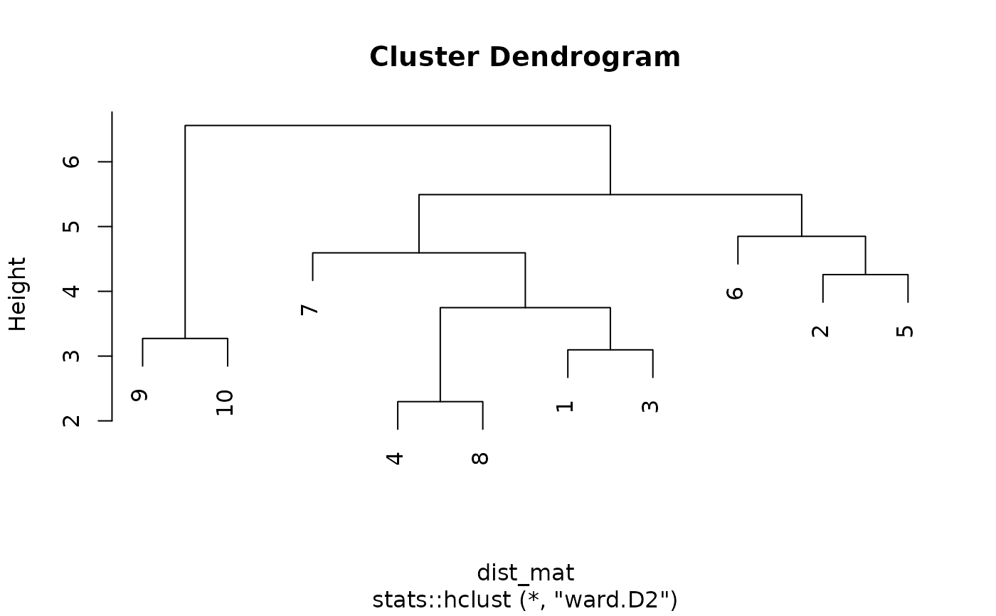
# Get full hclust object for plotting
hc <- get_analysis(tm, "row_hclust")
plot(hc)


# Multiple clusterings with different k
tm <- tm |>
  activate(rows) |>
  compute_hclust(k = 3, name = "gene_k3") |>
  compute_hclust(k = 5, name = "gene_k5")